Reworked the documentation and examples for the compute graph. |
3 years ago | |
|---|---|---|
| .. | ||
| docassets | 3 years ago | |
| CMakeLists.txt | 3 years ago | |
| PythonTest.mo | 3 years ago | |
| README.md | 3 years ago | |
| appnodes.py | 3 years ago | |
| custom.py | 3 years ago | |
| graph.py | 3 years ago | |
| main.py | 4 years ago | |
| output.wav | 3 years ago | |
| sched.py | 3 years ago | |
| test.dot | 4 years ago | |
| test.pdf | 4 years ago | |
README.md
Example 7
This is an example showing how a graph in in Python (not C) can interact with an OpenModelica model.
First you need to get the project AVH-SystemModeling from our ARM-Software repository.
Then, you need launch OpenModelica and choose Open Model.
Select AVH-SystemModeling/VHTModelicaBlock/ARM/package.mo
Then choose Open Model again and select PythonTest.mo.
You should see something like that in Open Modelica:
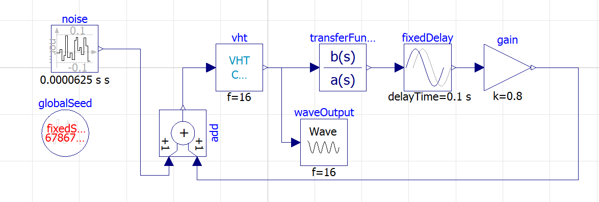
Customize the output path in the Wave node.
Refer to the Open Modelica documentation to know who to build and run this simulation. Once it is started in Modelica, launch the Python script in example7:
python main.py
You should see :
Connecting as INPUT
Connecting as OUTPUT
In Modelica window, the simulation should continue to 100%.
In the simulation window, you should be able to plot the output wav and get something like:
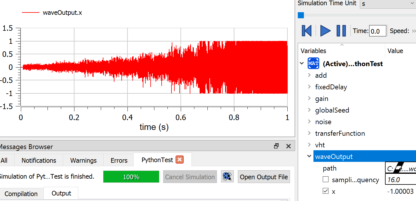
A .wav should have been generated so that you can listen to the result : A Larsen effect !
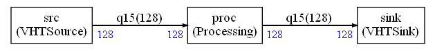
The Processing node in the compute graph is implemented in custom.py and is a gain computed with CMSIS-DSP Python wrapper
class Processing(GenericNode):
    def __init__(self,inputSize,outputSize,fifoin,fifoout):
        GenericNode.__init__(self,inputSize,outputSize,fifoin,fifoout)

    def run(self):

        i=self.getReadBuffer()
        o=self.getWriteBuffer()

        b=dsp.arm_scale_q15(i,0x6000,1)

        o[:]=b[:]

        return(0)
The gain has been chosen to create an instability.