The compute graph hierarchy (Python and C++) has been modified. It will break the code using the CG and the include and import will have to be modified. New function prepareForRunning is needed in CG nodes even if not used in static mode. Without this function, code using compute graph won't build. |
3 years ago | |
|---|---|---|
| .. | ||
| cg | 3 years ago | |
| documentation | 3 years ago | |
| examples | 3 years ago | |
| .gitignore | 4 years ago | |
| FAQ.md | 4 years ago | |
| MATHS.md | 4 years ago | |
| README.md | 3 years ago | |
| cg.scvd | 4 years ago | |
README.md
Compute Graph for streaming with CMSIS-DSP
Introduction
Embedded systems are often used to implement streaming solutions : the software is processing and / or generating stream of samples. The software is made of components that have no concept of streams : they are working with buffers. As a consequence, implementing a streaming solution is forcing the developer to think about scheduling questions, FIFO sizing etc ...
The CMSIS-DSP compute graph is a low overhead solution to this problem : it makes it easier to build streaming solutions by connecting components and computing a scheduling at build time. The use of C++ template also enables the compiler to have more information about the components for better code generation.
A dataflow graph is a representation of how compute blocks are connected to implement a streaming processing.
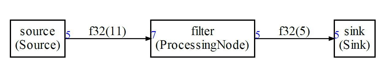
Here is an example with 3 nodes:
- A source
- A filter
- A sink
Each node is producing and consuming some amount of samples. For instance, the source node is producing 5 samples each time it is run. The filter node is consuming 7 samples each time it is run.
The FIFOs lengths are represented on each edge of the graph : 11 samples for the leftmost FIFO and 5 for the other one.
In blue, the amount of samples generated or consumed by a node each time it is called.
When the processing is applied to a stream of samples then the problem to solve is :
how the blocks must be scheduled and the FIFOs connecting the block dimensioned
The general problem can be very difficult. But, if some constraints are applied to the graph then some algorithms can compute a static schedule.
When the following constraints are satisfied we say we have a Synchronous Dataflow Graph:
- Static graph : graph topology is not changing
- Each node is always consuming and producing the same number of samples
In CMSIS-DSP, we are naming this a static flow.
The CMSIS-DSP Compute Graph Tools are a set of Python scripts and C++ classes with following features:
- A compute graph and its static flow can be described in Python
- The Python script will compute a static schedule and the FIFOs size
- A static schedule is:
- A periodic sequence of functions calls
- A periodic execution where the FIFOs remain bounded
- A periodic execution with no deadlock : when a node is run there is enough data available to run it
- The Python script will generate a Graphviz representation of the graph
- The Python script will generate a C++ implementation of the static schedule
- The Python script can also generate a Python implementation of the static schedule (for use with the CMSIS-DSP Python wrapper)
(There is no FIFO underflow or overflow due to the scheduling. If there are not enough cycles to run the processing, the real-time will be broken and the solution won't work But this problem is independent from the scheduling itself. )
Why it is useful
Without any scheduling tool for a dataflow graph, there is a problem of modularity : a change on a node may impact other nodes in the graph. For instance, if the number of samples consumed by a node is changed:
- You may need to change how many samples are produced by the predecessor blocks in the graph (assuming it is possible)
- You may need to change how many times the predecessor blocks must run
- You may have to change the FIFOs sizes
With the CMSIS-DSP Compute Graph (CG) Tools you don't have to think about those details while you are still experimenting with your data processing pipeline. It makes it easier to experiment, add or remove blocks, change their parameters.
The tools will generate a schedule and the FIFOs. Even if you don't use this at the end for a final implementation, the information could be useful : is the schedule too long ? Are the FIFOs too big ? Is there too much latency between the sources and the sinks ?
Let's look at an (artificial) example:
Without a tool, the user would probably try to modify the number of samples so that the number of sample produced is equal to the number of samples consumed. With the CG Tools we know that such a graph can be scheduled and that the FIFO sizes need to be 11 and 5.
The periodic schedule generated for this graph has a length of 19. It is big for such a small graph and it is because, indeed 5 and 7 are not very well chosen values. But, it is working even with those values.
The schedule is (the size of the FIFOs after the execution of the node displayed in the brackets):
source [ 5 0]
source [10 0]
filter [ 3 5]
sink [ 3 0]
source [ 8 0]
filter [ 1 5]
sink [ 1 0]
source [ 6 0]
source [11 0]
filter [ 4 5]
sink [ 4 0]
source [ 9 0]
filter [ 2 5]
sink [ 2 0]
source [ 7 0]
filter [ 0 5]
sink [ 0 0]
At the end, both FIFOs are empty so the schedule can be run again : it is periodic !
The latest version of the compute graph also supports dynamic scheduling.

How to use the static scheduler generator
First, you must install the CMSIS-DSP PythonWrapper:
pip install cmsisdsp
The functions and classes inside the cmsisdsp wrapper can be used to describe and generate the schedule.
To start, you can create a graph.py file and include :
from cmsisdsp.cg.static.scheduler import *
In this file, you can describe new type of blocks that you need in the compute graph if they are not provided by the python package by default.
Finally, you can execute graph.py to generate the C++ files.
The generated files need to include the ComputeGraph/cg/static/src/GenericNodes.h and the nodes used in the graph and which can be found in cg/static/nodes/cpp.
If you have declared new nodes in graph.py then you'll need to provide an implementation.
More details and explanations can be found in the documentation for the examples. The first example is a deep dive giving all the details about the Python and C++ sides of the tool:
- Example 1 : how to describe a simple graph
- Example 2 : More complex example with delay and CMSIS-DSP
- Example 3 : Working example with CMSIS-DSP and FFT
- Example 4 : Same as example 3 but with the CMSIS-DSP Python wrapper
Examples 5 and 6 are showing how to use the CMSIS-DSP MFCC with a synchronous data flow.
Example 7 is communicating with OpenModelica. The Modelica model (PythonTest) in the example is implementing a Larsen effect.
Example 8 is showing how to define a new custom datatype for the IOs of the nodes. Example 8 is also demonstrating a new feature where an IO can be connected up to 3 inputs and the static scheduler will automatically generate duplicate nodes.
Frequently asked questions:
There is a FAQ document.
Cyclo static scheduling
Beginning with the version 1.7.0 of the Python wrapper and version >= 1.12 of CMSIS-DSP, cyclo static scheduling has been added.
What is the problem it is trying to solve ?
Let's consider a sample rate converter from 48 kHz to 44.1 kHz.
For each input sample, on average it produces 44.1 / 48 = 0.91875 samples.
There are two ways to do this:
- One can observe that 48000/44100 = 160/147. So each time 160 samples are consumed, 147 samples are produced
- The number of sample produced can vary from one execution of the node to the other
In the first case, it is synchronous but you need to wait for 160 input samples before being able to do some processing. It is introducing a latency and depending on the sample rate and use case, this latency may be too big. We need more flexiblity.
In the second case, we have the flexibility but it is no more synchronous because the resampler is not producing the same amount of samples at each execution.
But we can observe that even if is is no more stationary, it is periodic. After consuming 160 samples the behavior should repeat.
One can use the resampler in the SpeexDSP project to test. If we decide to consume only 40 samples in input to have less latency, then the resampler of SpeexDSP will produce 37,37,37 and 36 samples for the first 4 executions.
And (40+40+40+40)/(37+37+37+36) = 160 / 147.
So the flow of data on the output is not static but it is periodic.
This is now supported in the CMSIS-DSP compute graph and on each IO one can define a period. For this example, it could be:
b=Sampler("sampler",floatType,40,[37,37,37,36])
Note that in the C++ class, the template parameters giving the number of samples produced or consumed on an IO cannot be used any more in this case. The value is still generated but now represent the maximum on a period.
And, in the run function you need to pass the number of sample read or written to the read and write buffer functions:
this->getWriteBuffer(nbOfSamplesForCurrentExecution)
For synchronous node, nothing is changed and they are coded as in the previous versions.
The drawback of cyclo static scheduling is that the schedule length is increased. If we take the first example with a source producing 5 samples and a node consuming 7 samples and if the source is replaced by another source producing [5,5] then it is not equivalent. In the first case we can have only one execution of the source. In the second case, the scheduling will always contain an even number of executions of the sources. So the schedule length will be bigger. But memory usage will be the same (FIFOs of same size).
Since schedule tend to be bigger with cyclo static scheduling, a new code generation mode has been introduced and is enabled by default : now instead of having a sequence of function calls, the schedule is coded by an array of number and there is a switch / case to select the function to be called.
Dynamic Data Flow
Versions of the compute graph corresponding to CMSIS-DSP Version >= 1.14.4 and Python wrapper version >= 1.10.0 are supporting a new dynamic / asynchronous mode.
With a dynamic flow, the flow of data is potentially changing at each execution. The IOs can generate or consume a different amount of data at each execution of their node (including no data).
This can be useful for sample oriented use cases where not all samples are available but a processing must nevertheless take place each time a subset of samples is available (samples could come from sensors).
With a dynamic flow and scheduling, there is no more any way to ensure that there won't be FIFO underflow of overflow due to scheduling. As consequence, the nodes must be able to check for this problem and decide what to do.
- A sink may decide to generate fake data in case of FIFO underflow
- A source may decide to skip some data in case of FIFO overflow
- Another node may decide to do nothing and skip the execution
- Another node may decide to raise an error.
With dynamic scheduling, a node must implement the function prepareForRunning and decide what to do.
3 error / status codes are reserved for this. They are defined in the header cg_status.h. This header is not included by default, but if you define you own error codes, they should be coherent with cg_status and use the same values for the 3 status / error codes which are used in dynamic mode:
CG_SUCCESS= 0 : Node can executeCG_SKIP_EXECUTION= -5 : Node will skip the executionCG_BUFFER_ERROR= -6 : Unrecoverable error due to FIFO underflow / overflow (only raised in pure function like CMSIS-DSP ones called directly)
Any other returned value will stop the execution.
The dynamic mode (also named asynchronous), is enabled with option : asynchronous
The system will still compute a scheduling and FIFO sizes as if the flow was static. We can see the static flow as an average of the dynamic flow. In dynamic mode, the FIFOs may need to be bigger than the ones computed in static mode. The static estimation is giving a first idea of what the size of the FIFOs should be. The size can be increased by specifying a percent increase with option FIFOIncrease.
For pure compute functions (like CMSIS-DSP ones), which are not packaged into a C++ class, there is no way to customize the decision logic in case of a problem with FIFO. There is a global option : asyncDefaultSkip.
When true, a pure function that cannot run will just skip the execution. With false, the execution will stop. For any other decision algorithm, the pure function needs to be packaged in a C++ class.
Duplicate nodes are skipping the execution in case of problems with FIFOs. If it is not the wanted behavior, you can either:
- Replace the Duplicate class by a custom one by changing the class name with option
duplicateNodeClassNameon the graph. - Don't use the automatic duplication feature and introduce your duplicate nodes in the compute graph
When you don't want to generate or consume data in a node, just don't call the functions getReadBuffer or getWriteBuffer for your IOs.
Options
Several options and be used to control the schedule generation. Some options are used by the scheduling algorithm and other options are used by the code generator:
Options for the graph
defaultFIFOClass (default = "FIFO")
Class used for FIFO by default. Can also be customized for each connection (connect of connectWithDelay call)
duplicateNodeClassName(default="Duplicate")
Prefix used to generate the duplicate node classes like Duplicate2, Duplicate3 ...
Options for the scheduling
memoryOptimization (default = False)
When the amount of data written to a FIFO and read from the FIFO is the same, the FIFO is just an array. In this case, depending on the scheduling, the memory used by different arrays may be reused if those arrays are not needed at the same time.
This option is enabling an analysis to optimize the memory usage by merging some buffers when it is possible.
sinkPriority (default = True)
Try to prioritize the scheduling of the sinks to minimize the latency between sources and sinks.
When this option is enable, the tool may not be able to find a schedule in all cases. If it can't find a schedule, it will raise a DeadLock exception.
displayFIFOSizes (default = False)
During computation of the schedule, the evolution of the FIFO sizes is generated on stdout.
dumpSchedule (default = False)
During computation of the schedule, the human readable schedule is generated on stdout.
Options for the code generator
debugLimit (default = 0)
When debugLimit is > 0, the number of iterations of the scheduling is limited to debugLimit. Otherwise, the scheduling is running forever or until an error has occured.
dumpFIFO (default = False)
When true, generate some code to dump the FIFO content at runtime. Only useful for debug.
In C code generation, it is only available when using the mode codeArray == False.
When this mode is enabled, the first line of the scheduler file is :
#define DEBUGSCHED 1
and it also enable some debug code in GenericNodes.h
schedName (default = "scheduler")
Name of the scheduler function used in the generated code.
prefix (default = "")
Prefix to add before the FIFO buffer definition. Those buffers are not static and are global. If you want to use several schedulers in your code, the buffer names used by each should be different.
Another possibility would be to make the buffer static by redefining the macro CG_BEFORE_BUFFER
Options for C Code Generation only
cOptionalArgs (default = "")
Optional arguments to pass to the C version of the scheduler function
codeArray (default = True)
When true, the scheduling is defined as an array. Otherwise, the list of function calls is generated.
The list of function call may be easier to read but if the schedule is long, it is not good for code size. In that case, it is better to encode the schedule as an array rather than a list of functions.
When codeArray is True, the option switchCase is taken into account.
switchCase (default = True)
codeArray must be true or this option is ignored.
When the schedule is encoded as an array, it can either be an array of function pointers (switchCase false) or an array of indexes for a state machine (switchCase true)
eventRecorder (default = False)
Enable the generation of CMSIS EventRecorder intrumentation in the code.
customCName (default = "custom.h")
Name of custom header in generated C code. If you use several scheduler, you may want to use different headers for each one.
postCustomCName (default = "")
Name of custom header in generated C code coming after all of the other includes.
genericNodeCName (default = "GenericNodes.h")
Name of GenericNodes header in generated C code. If you use several scheduler, you may want to use different headers for each one.
appNodesCName (default = "AppNodes.h")
Name of AppNodes header in generated C code. If you use several scheduler, you may want to use different headers for each one.
schedulerCFileName (default = "scheduler")
Name of scheduler cpp and header in generated C code. If you use several scheduler, you may want to use different headers for each one.
If the option is set to xxx, the names generated will be xxx.cpp and xxx.h
CAPI (default = True)
By default, the scheduler function is callable from C. When false, it is a standard C++ API.
CMSISDSP (default = True)
If you don't use any of the datatypes or functions of the CMSIS-DSP, you don't need to include the arm_math.h in the scheduler file. This option can thus be set to False.
asynchronous (default = False)
When true, the scheduling is for a dynamic / asynchronous flow. A node may not always produce or consume the same amount of data. As consequence, a scheduling can fail. Each node needs to implement a prepareForRunning function to identify and recover from FIFO underflows and overflows.
A synchronous schedule is used as start and should describe the average case.
This implies codeArray and switchCase. This disables memoryOptimizations.
Synchronous FIFOs that are just buffers will be considered as FIFOs in asynchronous mode.
FIFOIncrease (default 0)
In case of asynchronous scheduling, the FIFOs may need to be bigger than what is computed assuming a synchronous scheduling. This option is used to increase the FIFO size. It represents a percent increase.
For instance, a value of 10 means the FIFO will have their size updated from oldSize to 1.1 * oldSize which is (1 + 10%)* oldSize
asyncDefaultSkip (default True)
Behavior of a pure function (like CMSIS-DSP) in asynchronous mode. When True, the execution is skipped if the function can't be executed. If False, an error is raised.
If another error recovery is needed, the function must be packaged into a C++ class to implement a prepareForRun function.
Options for Python code generation only
pyOptionalArgs (default = "")
Optional arguments to pass to the Python version of the scheduler function
customPythonName (default = "custom")
Name of custom header in generated Python code. If you use several scheduler, you may want to use different headers for each one.
appNodesPythonName (default = "appnodes")
Name of AppNodes header in generated Python code. If you use several scheduler, you may want to use different headers for each one.
schedulerPythonFileName (default = "sched")
Name of scheduler file in generated Python code. If you use several scheduler, you may want to use different headers for each one.
If the option is set to xxx, the name generated will be xxx.py
Options for the graphviz generator
horizontal (default = True)
Horizontal or vertical layout for the graph.
displayFIFOBuf (default = False)
By default, the graph is displaying the FIFO sizes. If you want to know with FIFO variable is used in the code, you can set this option to true and the graph will display the FIFO variable names.
Options for connections
It is now possible to write something like:
g.connect(src.o,b.i,fifoClass="FIFOSource")
The fifoClass argument allows to choose a specific FIFO class in the generated C++ or Python.
Only the FIFO class is provided by default. Any new implementation must inherit from FIFObase<T>
How to build the examples
In folder ComputeGraph/example/build, type the cmake command:
cmake -DHOST=YES \
   -DDOT="path to dot.EXE" \
   -DCMSISCORE="path to cmsis core include directory" \
   -G "Unix Makefiles" ..
The Graphviz dot tool is requiring a recent version supporting the HTML-like labels.
If cmake is successful, you can type make to build the examples. It will also build CMSIS-DSP for the host.
If you don't have graphviz, the option -DDOT can be removed.
If for some reason it does not work, you can go into an example folder (for instance example1), and type the commands:
python graph.py
dot -Tpdf -o test.pdf test.dot
It will generate the C++ files for the schedule and a pdf representation of the graph.
Note that the Python code is relying on the CMSIS-DSP PythonWrapper which is now also containing the Python scripts for the Synchronous Data Flow.
To build the C examples:
- CMSIS-DSP must be built,
- the .cpp file contained in the example must be built
- the include folder
cg/static/srcmust be added
For example3 which is using an input file, cmake should have copied the input test pattern input_example3.txt inside the build folder. The output file will also be generated in the build folder.
example4 is like example3 but in pure Python and using the CMSIS-DSP Python wrapper (which must already be installed before trying the example). example4 is not built by the cmake. You'll need to go to the example4 folder and type:
python graph.py
python main.py
The first line is generating the schedule in Python. The second line is executing the schedule.
example7 is communicating with OpenModelica. You need to install the VHTModelica blocks from the VHT-SystemModeling project on our GitHub
Limitations
It is a first version and there are lots of limitations and probably bugs:
- The code generation is using Jinja template in
cg/static/templates. They must be cleaned to be more readable. You can modify the templates according to your needs ; - CMSIS-DSP integration must be improved to make it easier
- Some optimizations are missing
- Some checks are missing : for instance you can connect several nodes to the same io port. And io port must be connected to only one other io port. It is not checked by the script.
- The code is requiring a lot more comments and cleaning
- A C version of the code generator is missing
- The code generation could provide more flexibility for memory allocation with a choice between:
- Global
- Stack
- Heap
Default nodes
Here is a list of the nodes supported by default. More can be easily added:
- Unary:
- Unary function with header
void function(T* src, T* dst, int nbSamples)
- Unary function with header
- Binary:
- Binary function with header
void function(T* srcA, T* srcB, T* dst, int nbSamples)
- Binary function with header
- CMSIS-DSP function:
- It will detect if it is an unary or binary function.
- The name must not contain the prefix
armnor the the type suffix - For instance, use
Dsp("mult",CType(F32),NBSAMPLES)to usearm_mult_f32 - Other CMSIS-DSP function (with an instance variable) are requiring the creation of a Node if it is not already provided
- CFFT / ICFFT : Use of CMSIS-DSP CFFT. Currently only F32 and Q15
- Zip / Unzip : To zip / unzip streams
- ToComplex : Map a real stream onto a complex stream
- ToReal : Extract real part of a complex stream
- FileSource and FileSink : Read/write float to/from a file
- NullSink : Do nothing. Useful for debug
- StereoToMonoQ15 : Interleaved stereo converted to mono with scaling to avoid saturation of the addition
- Python only nodes:
- WavSink and WavSource to use wav files for testing
- VHTSDF : To communicate with OpenModelica using VHTModelica blocks