CMSIS-DSP/ComputeGraph/Introduction.md

Introduction

Embedded systems are often used to implement streaming solutions : the software is processing and / or generating stream of samples. The software is made of components that have no concept of streams : they are working with buffers. As a consequence, implementing a streaming solution is forcing the developer to think about scheduling questions, FIFO sizing etc ...

The CMSIS-DSP compute graph is a low overhead solution to this problem : it makes it easier to build streaming solutions by connecting components and computing a scheduling at build time. The use of C++ template also enables the compiler to have more information about the components for better code generation.

A dataflow graph is a representation of how compute blocks are connected to implement a streaming processing.

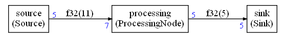
Here is an example with 3 nodes:

• A source
• A filter
• A sink

Each node is producing and consuming some amount of samples. For instance, the source node is producing 5 samples each time it is run. The filter node is consuming 7 samples each time it is run.

The FIFOs lengths are represented on each edge of the graph : 11 samples for the leftmost FIFO and 5 for the other one.

In blue, the amount of samples generated or consumed by a node each time it is called.

When the processing is applied to a stream of samples then the problem to solve is :

how the blocks must be scheduled and the FIFOs connecting the block dimensioned

The general problem can be very difficult. But, if some constraints are applied to the graph then some algorithms can compute a static schedule at build time.

When the following constraints are satisfied we say we have a Synchronous / Static Dataflow Graph:

• Each node is always consuming and producing the same number of samples (static / synchronous flow)

The CMSIS-DSP Compute Graph Tools are a set of Python scripts and C++ classes with following features:

• A compute graph and its static flow can be described in Python
• The Python script will compute a static schedule and the optimal FIFOs size
• A static schedule is:
  • A periodic sequence of functions calls
  • A periodic execution where the FIFOs remain bounded
  • A periodic execution with no deadlock : when a node is run there is enough data available to run it
• The Python script will generate a Graphviz representation of the graph
• The Python script will generate a C++ implementation of the static schedule
• The Python script can also generate a Python implementation of the static schedule (for use with the CMSIS-DSP Python wrapper)

There is no FIFO underflow or overflow due to the scheduling. If there are not enough cycles to run the processing, the real-time will be broken and the solution won't work. But this problem is independent from the scheduling itself.

Why it is useful

Without any scheduling tool for a dataflow graph, there is a problem of modularity : a change on a node may impact other nodes in the graph. For instance, if the number of samples consumed by a node is changed:

• You may need to change how many samples are produced by the predecessor blocks in the graph (assuming it is possible)
• You may need to change how many times the predecessor blocks must run
• You may have to change the FIFOs sizes

With the CMSIS-DSP Compute Graph (CG) Tools you don't have to think about those details while you are still experimenting with your data processing pipeline. It makes it easier to experiment, add or remove blocks, change their parameters.

The tools will generate a schedule and the FIFOs. Even if you don't use this at the end for a final implementation, the information could be useful : is the schedule too long ? Are the FIFOs too big ? Is there too much latency between the sources and the sinks ?

Let's look at an (artificial) example:

Without a tool, the user would probably try to modify the number of samples so that the number of sample produced is equal to the number of samples consumed. With the CG Tools we know that such a graph can be scheduled and that the FIFO sizes need to be 11 and 5.

The periodic schedule generated for this graph has a length of 19. It is big for such a small graph and it is because, indeed 5 and 7 are not very well chosen values. But, it is working even with those values.

The schedule is (the number of samples in the FIFOs after the execution of the nodes are displayed in the brackets):

source [ 5   0]
source [10   0]
filter [ 3   5]
sink   [ 3   0]
source [ 8   0]
filter [ 1   5]
sink   [ 1   0]
source [ 6   0]
source [11   0]
filter [ 4   5]
sink   [ 4   0]
source [ 9   0]
filter [ 2   5]
sink   [ 2   0]
source [ 7   0]
filter [ 0   5]
sink   [ 0   0]

At the end, both FIFOs are empty so the schedule can be run again : it is periodic !

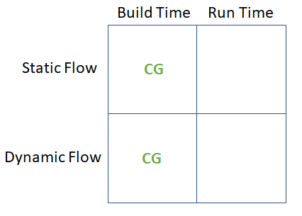
The compute graph is focusing on the synchronous / static case but some extensions have been introduced for more flexibility:

• A cyclo-static scheduling (nearly static)
• A dynamic/asynchronous mode

Here is a summary of the different configuration supported by the compute graph. The cyclo-static scheduling is part of the static flow mode.